Preface:
To train a network, we need to first evaluate the network, then think about why and how to optimize the network according to the evaluation results. This is a closed training loop.
1. How to Evaluate the Trained Network
The loss value is a parameter of your neural network that enables us to perform evaluation. This parameter reflects the gap between the results obtained by your trained network and the expected or “correct” value. Check how the loss curve changes as the number of iterations increases, this helps us to check whether the training is overfitted and whether the learning rate is too small.
1.1 Save the .log file during training
nohup ./darknet detector train khadas_ai/khadas_ai.data khadas_ai/yolov3-khadas_ai.cfg_train darknet53.conv.74 -dont_show > train.log 2>&1 &
1.2 Use the extract_log.py script to convert your .log file to the appropriate format
import inspect
import os
import random
import sys
def extract_log(log_file,new_log_file,key_word):
    with open(log_file, 'r') as f:
      with open(new_log_file, 'w') as train_log:
  #f = open(log_file)
    #train_log = open(new_log_file, 'w')
        for line in f:
          if 'Syncing' in line:
            continue
          if 'nan' in line:
            continue
          if 'Region 82 Avg' in line:
            continue
          if 'Region 94 Avg' in line:
            continue
          if 'Region 106 Avg' in line:
            continue
          if 'total_bbox' in line:
            continue
          if 'Loaded' in line:
            continue
          if key_word in line:
            train_log.write(line)
    f.close()
    train_log.close()

def extract_log2(log_file,new_log_file,key_word):
    with open(log_file, 'r') as f:
      with open(new_log_file, 'w') as train_log:
  #f = open(log_file)
    #train_log = open(new_log_file, 'w')
        for line in f:
          if 'Syncing' in line:
            continue
          if 'nan' in line:
            continue
          if 'Region 94 Avg' in line:
            continue
          if 'Region 106 Avg' in line:
            continue
          if 'total_bbox' in line:
            continue
          if 'Loaded' in line:
            continue
          if 'IOU: 0.000000' in line:
            continue
          if key_word in line:
            del_num=line.replace("v3 (mse loss, Normalizer: (iou: 0.75, obj: 1.00, cls: 1.00) Region 82 Avg (", "")
            train_log.write(del_num.replace(")", ""))
    f.close()
    train_log.close()
extract_log('train.log','train_log_loss.txt','images')
extract_log2('train.log','train_log_iou.txt','IOU')
After running the extract_log.py script, it will parse the loss line and IOU line of the .log file to get two .txt files.
1.3 Use the train_loss_visualization.py script to draw the loss curve:
import pandas as pd
import numpy as np
import matplotlib.pyplot as plt
#%matplotlib inline

lines =18798    #Change to self generated Number of rows in train_log_loss.txt

#Adjusting the following two sets of numbers will help you view the details of the drawing
start_ite = 250 #Ignore Number of all lines starting in train_log_loss.txt
end_ite = 6000 #Ignore Number of all lines ending in train_log_loss.txt
result = pd.read_csv('train_log_loss.txt', skiprows=[x for x in range(lines) if ((x<start_ite) |(x>end_ite))] ,error_bad_lines=False, names=['loss', 'avg loss', 'rate', 'seconds', 'images'])
result.head()

result['loss']=result['loss'].str.split(' ').str.get(1)
result['avg']=result['avg loss'].str.split(' ').str.get(1)
result['rate']=result['rate'].str.split(' ').str.get(1)
result['seconds']=result['seconds'].str.split(' ').str.get(1)
result['images']=result['images'].str.split(' ').str.get(1)
result.head()
result.tail()

# print(result.head())
# print(result.tail())
# print(result.dtypes)
print(result['loss'])
#print(result['avg'])
#print(result['rate'])
#print(result['seconds'])
#print(result['images'])

result['loss']=pd.to_numeric(result['loss'])
result['avg']=pd.to_numeric(result['avg'])
result['rate']=pd.to_numeric(result['rate'])
result['seconds']=pd.to_numeric(result['seconds'])
result['images']=pd.to_numeric(result['images'])
result.dtypes


fig = plt.figure()
ax = fig.add_subplot(1, 1, 1)
ax.plot(result['loss'].values,label='avg_loss')
ax.legend(loc='best')
ax.set_title('The loss curves')
ax.set_xlabel('batches')
fig.savefig('avg_loss')
Modify the file train_loss_visualization.py to skip rows within the train_log_loss.txt file as needed: skiprows=[x for x in range(lines) if ((x<start_ite) |(x>end_ite))]
Running train_loss_visualization.py will generate a picture avg_loss.png in the path where the script is located.
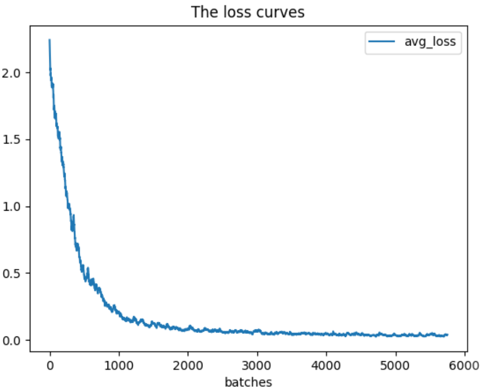
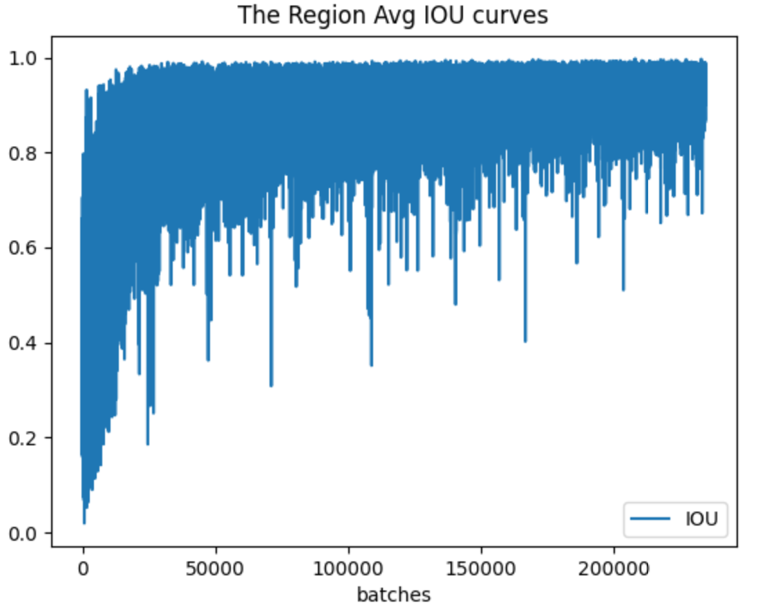
By analyzing the loss curve, we can appropriately change the learning rate of our neural network to more quickly converge on our expected value. In addition to visualizing loss, you can also visualize parameters such as the Avg IOU. The script train_iou_visualization.py can be used in the same way as train_loss_visualization.py. The script train_iou_visualization.py is as follows:
import pandas as pd
import numpy as np
import matplotlib.pyplot as plt
#%matplotlib inline

lines = 234429    #Change to self generated Number of rows in train_log_iou.txt

#Adjusting the following two sets of numbers will help you view the details of the drawing
start_ite = 1 #Ignore Number of all lines starting in train_log_iou.txt
end_ite = 234429 #Ignore Number of all lines ending in train_log_iou.txt
result = pd.read_csv('train_log_iou.txt', skiprows=[x for x in range(lines) if ((x<start_ite) |(x>end_ite)) ] ,error_bad_lines=False, names=['IOU', 'count', 'class_loss', 'iou_loss', 'total_loss'])
result.head()

result['IOU']=result['IOU'].str.split(': ').str.get(1)
result['count']=result['count'].str.split(': ').str.get(1)
result['class_loss']=result['class_loss'].str.split('= ').str.get(1)
result['iou_loss']=result['iou_loss'].str.split('= ').str.get(1)
result['total_loss']=result['total_loss'].str.split('= ').str.get(1)
result.head()
result.tail()

# print(result.head())
# print(result.tail())
# print(result.dtypes)
print(result['IOU'])
#print(result['count'])
#print(result['class_loss'])
#print(result['iou_loss'])
#print(result['total_loss'])

result['IOU']=pd.to_numeric(result['IOU'])
result['count']=pd.to_numeric(result['count'])
result['class_loss']=pd.to_numeric(result['class_loss'])
result['iou_loss']=pd.to_numeric(result['iou_loss'])
result['total_loss']=pd.to_numeric(result['total_loss'])
result.dtypes

fig = plt.figure()
ax = fig.add_subplot(1, 1, 1)
ax.plot(result['IOU'].values,label='IOU')
ax.legend(loc='best')
ax.set_title('The Region Avg IOU curves')
ax.set_xlabel('batches')
fig.savefig('Avg_IOU')
Running train_iou_visualization.py will generate a picture called Avg_IOU.png in the path where the script is located.
-
Region Avg IOU: This is the intersection of the “predicted bounding box” with your “labeled bounding box”, divided by their union. Obviously, the larger the obtained value, the better the prediction result.
2. View the Recall Value for your Neural Network
Recall is the ratio of the number of correctly identified positive samples to the number of all positive samples in the test set. Obviously, the larger the value, the better the prediction result.
./darknet detector recall khadas_ai/khadas_ai.data khadas_ai/yolov3-khadas_ai.cfg_train khadas_ai/yolov3-khadas_ai_last.weights
The final log is as follows:
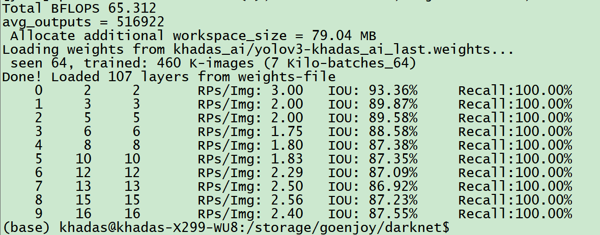
The output format is:
Number Correct Total Rps/Img IOU Recall
The specific explanations are as follows:
-
Number: Indicates the number of pictures processed. -
Correct: The steps to calculate this value are as follows: throw a picture into the network, and the network will predict many bounding boxes. Each bounding box has its own confidence or “probability of being correct”. The bounding box with a probability greater than the threshold value means that it has been labelled correctly. Calculate theIOUand find the bounding box with the largestIOU. If this maximum value is greater than the presetIOU threshold, correct plus one. -
Total: Indicates the actual number of bounding boxes. -
Rps/img: Indicates the average number of bounding boxes predicted for each picture. -
IOU: This is the intersection of the “predicted bounding box” with your “labeled bounding box”, divided by their union. Obviously, the larger the obtained value, the better the prediction result. -
Recall: Refers to the number of detected objects divided by the number of all labeled objects. We can also see from the code that it is the value ofCorrectdivided byTotal.